ABSTRACT

This is part of a multi-year project carried out along side Veronica Wharton, Ellie Pavlick (now professor at Brown University), Anne Cocos , supervised by Chris Callison-Burch. Adjectives such as fine, good, great, and out- standing are semantically similar but differ in intensity (i.e., fine, good, great). Understanding such intensity differences is crucial for fluid natural language interface. Leveraging the ParaPhrase database, we developed a pipeline to learn the relative relationship among adjectives. In particular, using the data base we constructed a directed graph where vertices are adjectives and edges are adverbs, so that if there is an edge from vertex s to t with label u, then the string “u s” is a ParaPhrase of the string “t”. Then we developed an l1-penalized logistic regression model that inferred the relative strength of adjectives based on relationship with their neighbors. The ground truth is procured by Amazon mechanical turks. Preliminary tests show that our approach outperform the state of the art by significant margins measured by both pairwise accuracy and Kendall’s tau score.

INTRODUCTION

One of the most exciting trends in the next decade is ambient computing: an ongoing, multi-modal augmented experience of the world. Ambient computing promises technology will fade into the background, and people will once again occupy the foreground in our lives. One gateway to ambient computing is voice. Presently, voice-driven consumer products such as Siri, Amazon Alexa, and Google Home has already made considerable inroads into many of our lives. In the future, a more engaging and useful dialogue system requires an even more sophisticated understanding of the endless subtlety of human speech. Modern dialogue systems rely on rich lexical knowledge base for subtlety. And one such subtlety is adjectives that are supposedly synonymous but actually differ in intensity, for example a good burger is different than an excellent burger. However, commonly used lexical resources such as WordNet do not disambiguate the varying intensity among synonymous adjectives.

Prior Work

Bansal and de Melo used pairwise co-occurrence of adjectives around manually procured patterns that signify the adjectives relative strength. For example if good co-occur with great in the pattern "good but not great", then we suspect good is less intense than great (see paper link for the rest of the patterns). Then they counted the frequency of said patterns for each pair of adjectives in the Google N-grams corpus. They encountered two primary challenges:

1. Data sparsity: since the patterns are two to three words long, a pattern with two adjectives is four to five words long, any phrase of such length is rare in corpus.
2. Contradictory data: language use is noisy and often times data suggest a word is both weaker and strong than another word.

Bansal and de Melo solved the problem by aggregating the data in an integer linear program (ILP) formulation that look for the most likely ordering given the data, subject to transitivity constraints. That is if s is less intense than t, and t less intense than r, then s is less intense than r. They procured 93 clusters, with two to seven words in each cluster, and procured labels by ranking each cluster using Amazon Mechanical Turks. Five of the clusters were used to develop the algorithm, while the remaining 88 were held out as the test set. Their formulation outperformed the previous state of the art by 46%. However, we replicated and applied the ILP algorithm to a newly procured cluster and saw their method failed outright. Upon closer inspection we found that it failed because of data sparsity in Google N-Gram, segmenting the errors it became clear that Bansal’s formulation performed acceptably when more than 2/3 of all pairs in a cluster witnessed some comparison in data, but most of the words in the clusters we procured did not appear in the N-Gram corpus with the linguistic patterns they used. Instead of collecting more n-grams or finding new patterns, we reposed the question as a machine learning problem, where we learn the most likely ordering given two words and their respective neighbors in a newly constructed data set from the Paraphrase Database.

DATA SET

In this section we describe the motivation of the paraphrase database (PPDB), and the directed graph of adjective and adverbs constructed using PPDB.

Paraphrase Database (PPDB)

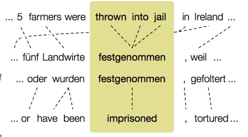
Paraphrases are different textual realizations of the same meaning and are valuable for a variety of downstream natural language processing (NLP) tasks such as textual entailment, measuring semantic similarity of texts, monolingual alignment, natural language generation, and improving lexical embeddings. The paraphrase database is a collection of over 220 million paraphrase patterns, comprised of 73 million phrasal and 8 million lexical paraphrases, and 140 million paraphrase patterns that capture meaning equivalent syntactic transformations. The paraphrases are extracted from bilingual parallel corpora of over 100 million sentence pairs and over 2 billion English words. Specifically, if two English strings translate to the same foreign string (commonly called a pivot string) in some text, then it is assumed that they have the same meaning. PPDB provides a set of paraphrases for each string and their associated distributional similarity, very loosely interpreted as a confidence score of how likely one utterance is a paraphrase of another. The similarity is computed as the cosine distance between the feature representation of the two phrases, where the feature set is comprised of n-grams and syntactical features.

Paraphrase Graph

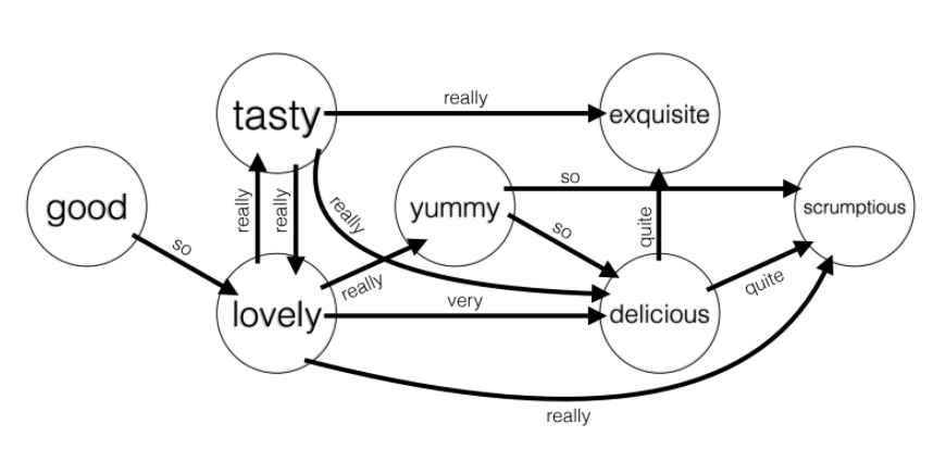
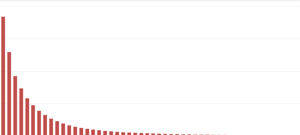
Inspecting PPDB, we find a litany of (adj, adv adj) paraphrase pairs that could be valuable in ranking adjectives, for example (“great”, “very good”) and (“great”, “extremely good”). Furthermore, we hypothesized that both the frequency and intensity of adverbs (ie very vs extremely) modifying the adjective are informative features when ranking adjectives. This intuition motivated the construction of the Adverb Paraphrase Graph where the vertices are adjectives, and the directed edges are adverbs, so that if there is an edge from vertex s to t with label u, then the string u s is a paraphrase of t. We bootstrapped the graph by manually selecting base, comparative, and superlative adjective triplets, and and pruned PPDB for the adverbs that modified the weaker word in the triplet so that the clause is a paraphrase of the stronger adjective. We then compiled all (adj_1 adj_2; adv) triplets from the PPDB given the adverbs we have collected. Overall the graph has 18,936 edges, covering 2,745 adjectives modified by 544 unique adverbs. On a practical note, upon closer inspection it became clear that some adverbs de-intensified the adjective (“somewhat”) while others intensified it (“very”), however analysis shows that the overwhelming majority of adverbs appear as intensifiers, thus removed the de-intensifiers from the graph.

N-Gram Graph

We noted that the directed graph formulation can be readily applied to N-Graph data as well, in this case the pattern “good but not great” could correspond to the tuple (good, but not great), whereby the utterance “but not” de-intensify the adjective “great”. In the interest of simplicity we invert the edge so that the triplet is actually (good, great; but not) in keeping with the convention that the source of the edge is weaker than the target under the edge label. The N-gram graph has 36,8439 edges, but only covers 178 of the adjectives we found in Paraphrase Graph.

Ground Truth

We constructed 81 adjective clusters and ranked them using Mechanical Turks. On average there are 2.8 words per cluster, and no cluster exceeded four words.

PROBLEM FORMULATION

Total Ordering

Similar to Bansal, we separate the ranking task into pairwise ordering and total ranking. In total ranking, we assume a generative process where a coin are tossed independently between vertices, and directed edges are placed according to how the coin lands. Thus the most likely ordering of adjective in a cluster is equivalent to the most likely set of edges among the vertices, subject to transitivity constraints. For example, suppose we have vertices s, t, and r, then there are six possible consistent orderings:

1. s < t < r
2. s < r < t
3. t < s < r
4. t < r < s
5. r < s < t
6. r < t < s

Furthermore, suppose we have s < t < r, then a subgraph corresponding to this ordering would be the set of pairs: {(s, t), (s, r), and (t, r)}, where each pair correspond to a Bernoulli variable. Thus we enumerate all possible total orderings (tractable because the clusters are relatively small), and then computing the likelihood of each ranked pair. Finally, per independence assumption the pairwise probability is multiplied to arrive at the likelihood of the final ordering, and the most likely one is chosen.

Pairwise Ordering

Now we must find a pairwise ranking algorithm that is robust to noise and data sparsity, and outputs a likelihood of the rank. The directed graphs makes us suspect that the relationship between words does to simply depend on their local connectivity, but that of its connectivity to their neighbors as well. This process could conceivably recurse outward, which inspired our initial attempt at ranking adjectives using well-known network centrality measures such as PageRank and Personalized PageRank. This formulation is stimulating but results proved this intuition to be misguided. Instead, we opted for frequency based estimation where the Bernoulli parameter of each edge is the empirical likelihood computed by the in-degree divided by the total degree. If two words are to be compared but their comparisons are not observed, then we employ a machine learning approach where the local connectivity of the graph is used as feature representation for the words. In particular we experimented with lasso and ridge regression where the input is some representation of the adjective pair (s, t), and the binary output is 1 if s is less than t, and 0 otherwise. We used the base, superlative and comparative set of comparisons as training data. Empirically speaking, the best representation of the adjective pair (s, t) is the concatenation of the top 10 most connected adjectives neighboring s and t, where each neighbor is represented by a value in [0,1] computed as in degree divided by total degree of the adjective, note this is conceptually different than the representation of the edges. The feature vector is interesting because:

• The connectivity information of a vertex to its neighbors is not used
• The less connected neighbors are not considered

This makes the representation of (s, t) robust to noise and data sparsity. Since the features are easily interpretable, it’s curious to read the model as stating that the neighbors of words are very informative to how strong the word is emotionally. Because the total ranking system demands a probability, we experiment with two methods. As a baseline we arbitrarily assign a value (1/2 + epsilon) for some very small epsilon if logistic regression decides s is less than t, and 1/2 - epsilon otherwise. Note in the case where there is absolutely not data, we output 1/2, interpreted as “do not know.” Next, we define a formal variant of the baseline where we use beta priors of various confidence levels, and update the belief after observing data.

RESULTS AND DISCUSSION

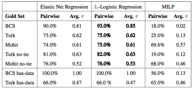
We measured the quality of our ranking using pairwise accuracy, defined as the fraction of pairs that is correctly classified. And Kendall's-τ, which measures the total number of pairwise inversions. We trained our model on the paraphrase graph alone, the N-gram graph alone, and both graphs combined. Curiously we found that PPDB has great data coverage over the set of adjectives in our test set, but poor coverage over Bansal's test set. Similarly Bansal's dataset does not cover our test set at all. In figure 5 we report the logistic regression model trained on the combine graph only. The model outperforms Bansal's MILP method across all test sets and both measures, demonstrating the efficacy of incorporating PPDB and N-gram data into a machine-learning based prediction system.

CONCLUSION

The fundamental hypothesis underlying all methods is that there is a positive relationship between how words are used on average in the context of intensifiers such as adverbs or N-gram patterns, and how an annotator ranks pairs of such words in isolation. The fact that all successful methods we have seen so far achieved close to or above 70% pairwise accuracy confirms this hypothesis. However, we must caution those who wish to improve upon this results, inter-annotator accuracy on Mohit’s set is 78%. In fact, many of the rankings are subjective and we do not believe it is meaningful to achieve aim for accuracy higher than 90%. Some of the clusters contained adjectives that are not necessarily synonymous, and thus it is difficult for the annotators to agree on a ranking (independently). Therefore the best way forward is actually to procure "better" clusters where adjectives can fall on a similar scale. There are two ways to improve the quality of each cluster: prune the clusters for synonyms, and resist the temptation for large clusters. The first suggestion is self explanatory, since none of the models account for synonyms, clusters that contain words annotators would consider to be synonyms will unfairly depress the score. Eschewing large clusters is important because the larger the cluster, the more likely polysemy wills confuse the annotator.